About this article
The pipeline code, data cleaning decisions, exploratory analysis, machine learning experiments, and GPU setup described here were all designed and implemented by the human author. Claude’s contributions were: reading the source code and notebook in full, writing the narrative sections before the EDA (“Architecture”, “Fetching with a Cache”, “Cleaning the Data”), extracting the charts from the notebook’s embedded PNG data, and writing the explanatory prose between notebook cells in the EDA section. Inline collaboration notes appear at specific moments throughout to make the division of work explicit.
Ireland maintains a public register of every residential property sale that has taken place in the country since 2010. The Residential Property Price Register (RPPR) is published by the Property Services Regulatory Authority and updated weekly. It contains the sale date, address, county, Eircode, price paid, whether the price was VAT-exclusive, and whether the sale was at full market value.
Nearly 730,000 transactions spanning fifteen years of the Irish housing market — that is a genuinely interesting dataset, and it is sitting there as a public ZIP file waiting to be downloaded.
This project builds an automated pipeline to fetch, clean, and load that data, then uses a Jupyter notebook for exploratory analysis and machine learning to fill gaps in the data.
Architecture
The pipeline has two stages, orchestrated by Apache Airflow:
fetch_dataset → process_data
fetch_dataset downloads the ZIP archive from the RPPR website, extracts the CSV, and caches it locally with a 24-hour TTL to avoid hammering the source on every run. The DAG runs on a weekly schedule (@weekly), matching the RPPR update frequency.
process_data reads that CSV, runs the cleaning pipeline, and writes the result to a Parquet file. Parquet is column-oriented and significantly faster to query than CSV for the kind of aggregations we do in the notebook.
The whole thing runs in Docker. The docker-compose.yml brings up:
- PostgreSQL — Airflow metadata database
- Redis — Celery broker
- airflow-init — one-shot container that initialises the database and creates the admin user
- webserver — the Airflow UI on port 8080
- scheduler — DAG trigger and task queuing
- worker — Celery worker that executes the Python tasks
The Airflow image is built on top of apache/airflow:2.7.3-python3.11 with our dependencies layered on. The DAG file and source modules are bind-mounted into the running containers, so changes take effect without a rebuild during development.
fetch_task = PythonOperator(
    task_id='fetch_dataset',
    python_callable=fetch_dataset_task,
    op_kwargs={'cache_ttl_hours': 24},
    dag=dag,
)

process_task = PythonOperator(
    task_id='process_data',
    python_callable=process_data_task,
    dag=dag,
)

fetch_task >> process_task
Fetching with a Cache
The source file is a ZIP hosted on the RPPR website. The fetch module checks whether a local copy exists and how old it is before deciding whether to download:
def check_cache_validity(file_path: str, cache_ttl_hours: int) -> bool:
    if not os.path.exists(file_path):
        return False
    age = datetime.now() - datetime.fromtimestamp(os.path.getmtime(file_path))
    return age < timedelta(hours=cache_ttl_hours)
If the cache is still valid, the download is skipped entirely. This matters because the weekly schedule will hit the cache on most task retries, and being a good citizen toward public data sources is always worth a few lines of code.
You can force a re-download by setting cache_ttl_hours=0 when triggering the task manually:
docker-compose exec scheduler \
  airflow tasks test rppr_data_pipeline fetch_dataset --
Cleaning the Data
Collaboration: The decisions in this section — which rows to remove, how to handle encoding failures, what VAT rate to apply — are entirely the author’s, documented as inline comments in
src/process/pipeline.py. Claude read those comments to write the explanations below. The comments in the pipeline are unusually thorough, which made Claude’s job here straightforward.
The raw CSV has some rough edges. The cleaning pipeline (src/process/pipeline.py) addresses each one deliberately.
Price parsing. Prices arrive as strings like "€450,000". The euro sign is stripped, the comma thousands-separator is removed, and the column is cast to numeric.
VAT normalisation. Some new-build sales are recorded as VAT-exclusive prices. These are adjusted upward by 13.5% (the applicable rate for residential construction) so every price in the processed dataset is comparable:
df.loc[df['VAT Exclusive'] == 'Yes', 'Price'] *= 1.135
df.loc[df['VAT Exclusive'] == 'Yes', 'VAT Exclusive'] = 'No'
Non-market sales. Transactions flagged as “Not Full Market Price” are removed. These are typically transfers between family members or other non-arm’s-length deals that would distort any price analysis.
Unicode corruption in Irish-language descriptions. Some rows in the Description of Property column contain garbled text — Irish-language property descriptions that were corrupted by a character encoding mismatch. These represent approximately 0.006% of all rows. Since the categories of interest (new dwelling vs. second-hand dwelling) are cleanly encoded in English, the corrupted rows are dropped and their categories removed from the categorical index.
Date decomposition. The original date column (Date of Sale (dd/mm/yyyy)) is parsed and then split into three separate columns — Year_of_Sale, Month_of_Sale, and Day_of_Sale — stored as integers. This makes grouping and plotting by year or month straightforward without any further processing in the notebook.
Deduplication. Exact duplicate rows are removed.
The result is written to data/processed/processed_data.parquet.
Exploratory Data Analysis
Collaboration: Everything inside a code block from this point onwards — including all markdown cell text — is the author’s verbatim work from
exploration.ipynb. The prose that appears between sections (like this note) is Claude’s, written by reading the outputs and inferring what they mean in context. The charts were extracted by Claude by parsing the notebook’s JSON file, locating theimage/pngkey in each cell’soutputsarray, and base64-decoding the embedded PNG data into static files.
Loading the data
import pandas as pd
import pyarrow as pa
import pyarrow.parquet as pq

rppr = pq.read_table(
    '/home/gary/git/rppr-ml/rppr-ml/data/processed/processed_data.parquet'
).to_pandas()
rppr.info()
<class 'pandas.core.frame.DataFrame'>
Index: 729783 entries, 0 to 769822
Data columns (total 11 columns):
 #   Column                     Non-Null Count   Dtype
---  ------                     --------------   -----
 0   Address                    729783 non-null  string
 1   County                     729783 non-null  category
 2   Eircode                    729783 non-null  string
 3   Price                      729783 non-null  float64
 4   Not_Full_Market_Price      729783 non-null  category
 5   VAT_Exclusive              729783 non-null  category
 6   Description_of_Property    729783 non-null  category
 7   Property_Size_Description  51135 non-null   category
 8   Year_of_Sale               729783 non-null  int32
 9   Month_of_Sale              729783 non-null  int32
 10  Day_of_Sale                729783 non-null  int32
dtypes: category(5), float64(1), int32(3), string(2)
memory usage: 34.1 MB
729,783 records, 34 MB in memory. Property_Size_Description immediately stands out: only 51,135 non-null values out of 729,783 total.
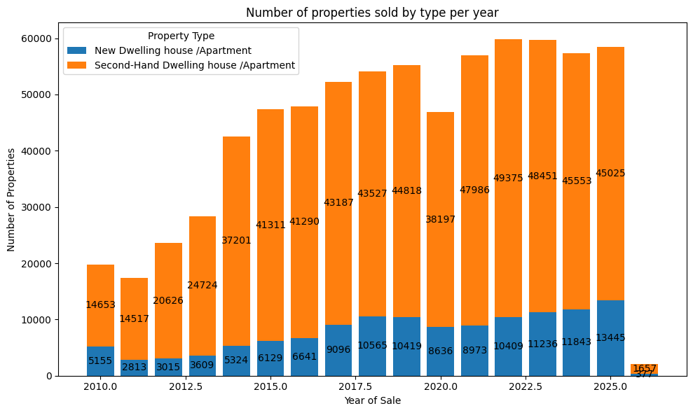
Sales by property type per year
Let’s take a look at some visual representations of the data for the whole country. I have used information from the matplotlib/seaborn website/documentation to assist with creating charts.
import matplotlib.pyplot as plt
import numpy as np

# Group and pivot the data
grouped_year_desc = rppr.groupby(
    ['Year_of_Sale', 'Description_of_Property'], observed=False
).size().unstack(fill_value=0)

# Sort by year
grouped_year_desc = grouped_year_desc.sort_index()

# Set up the plot
fig, ax = plt.subplots(figsize=(10, 6))
bottom = np.zeros(len(grouped_year_desc))

# Loop through each property description and plot it
for desc in grouped_year_desc.columns:
    counts = grouped_year_desc[desc].values
    p = ax.bar(grouped_year_desc.index, counts, label=desc, bottom=bottom)
    bottom += counts
    ax.bar_label(
        p, label_type='center',
        labels=[str(int(c)) if c > 0 else '' for c in counts]
    )

# Formatting
ax.set_title('Number of properties sold by type per year')
ax.set_xlabel('Year of Sale')
ax.set_ylabel('Number of Properties')
ax.legend(title='Property Type')
plt.tight_layout()
plt.show()
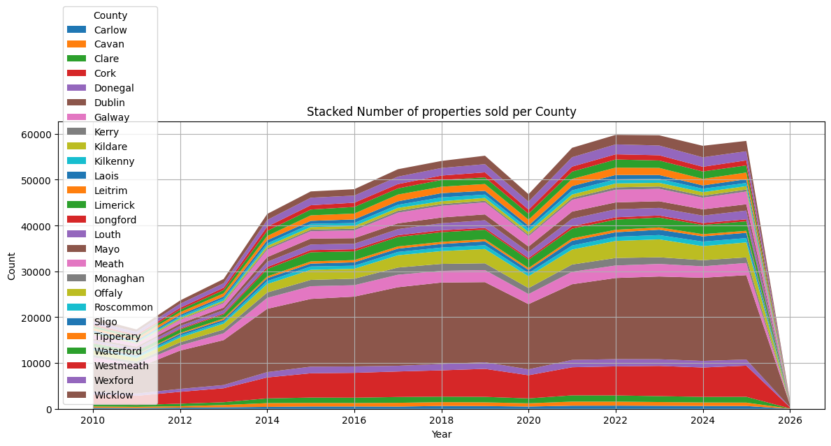
Sales by county — all counties
Despite slight dips in 2011, 2020, and 2024, the general trend has been an increase in sales, predominantly second-hand properties. Where are most new properties being sold?
grouped_new_by_year_county = rppr.groupby(
    ['Year_of_Sale', 'County'], observed=False
).size().reset_index(name='count')
pivot_grouped_new = grouped_new_by_year_county.pivot_table(
    index='Year_of_Sale', columns='County',
    values='count', aggfunc='sum', observed=False
)
pivot_grouped_new = pivot_grouped_new.sort_index()
plt.figure(figsize=(12, 6))
plt.stackplot(
    pivot_grouped_new.index, pivot_grouped_new.T.values,
    labels=pivot_grouped_new.columns
)
plt.legend(loc='lower left', title='County')
plt.xlabel("Year")
plt.ylabel("Count")
plt.title("Stacked Number of properties sold per County")
plt.tight_layout()
plt.grid(True)
plt.show()
Top 10 counties — new sales
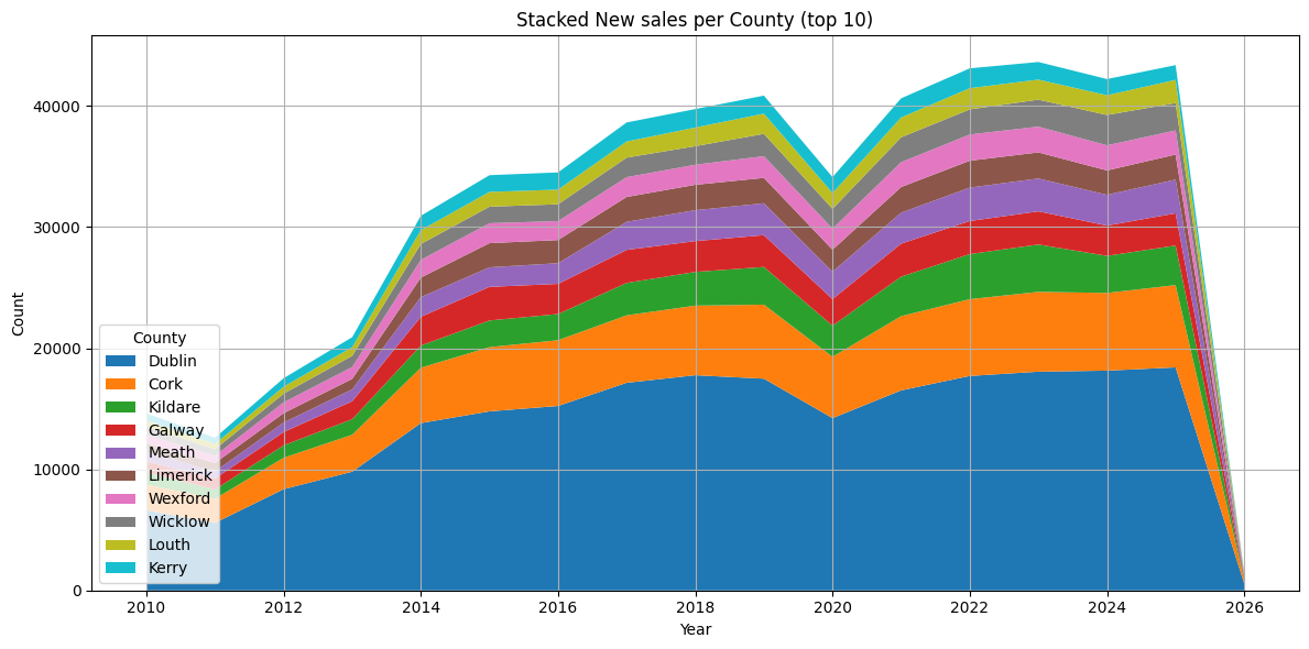
It’s a bit hard to be sure because some of the colours appear to be repeating (due to the number of trends). I will limit this to the top 10 counties to make it easier to see where most market activity has been.
county_totals_new = pivot_grouped_new.sum(axis=0)
top_10_counties_new = county_totals_new.nlargest(10).index
pivot_grouped_new_top10 = pivot_grouped_new[top_10_counties_new]
pivot_grouped_new_top10 = pivot_grouped_new_top10.sort_index()
plt.figure(figsize=(12, 6))
plt.stackplot(
    pivot_grouped_new_top10.index, pivot_grouped_new_top10.T.values,
    labels=pivot_grouped_new_top10.columns
)
plt.legend(loc='lower left', title='County')
plt.xlabel("Year")
plt.ylabel("Count")
plt.title("Stacked New sales per County (top 10)")
plt.tight_layout()
plt.grid(True)
plt.show()
Top 10 counties — second-hand sales
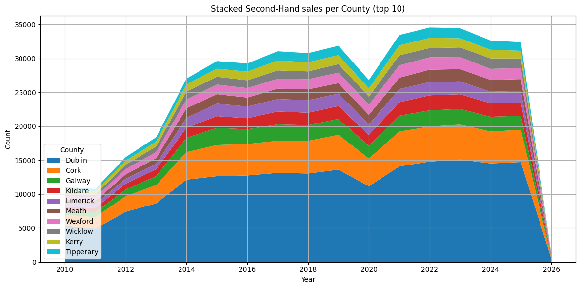
That’s better. No real surprise that Dublin and Cork are top. What about second-hand properties?
grouped_second_hand_by_year_county = rppr[
    rppr['Description_of_Property'] == 'Second-Hand Dwelling house /Apartment'
].groupby(['Year_of_Sale', 'County'], observed=False).size().reset_index(name='count')
pivot_grouped_second_hand = grouped_second_hand_by_year_county.pivot_table(
    index='Year_of_Sale', columns='County',
    values='count', aggfunc='sum', observed=False
)
pivot_grouped_second_hand = pivot_grouped_second_hand.sort_index()
county_totals_second_hand = pivot_grouped_second_hand.sum(axis=0)
top_10_counties_second_hand = county_totals_second_hand.nlargest(10).index
pivot_grouped_second_hand_top10 = pivot_grouped_second_hand[top_10_counties_second_hand]
pivot_grouped_second_hand_top10 = pivot_grouped_second_hand_top10.sort_index()
plt.figure(figsize=(12, 6))
plt.stackplot(
    pivot_grouped_second_hand_top10.index,
    pivot_grouped_second_hand_top10.T.values,
    labels=pivot_grouped_second_hand_top10.columns
)
plt.legend(loc='lower left', title='County')
plt.xlabel("Year")
plt.ylabel("Count")
plt.title("Stacked Second-Hand sales per County (top 10)")
plt.tight_layout()
plt.grid(True)
plt.show()
The Property Size Problem
Dublin and Cork are top again. Interesting that Louth is in the top 10 for New sales, but not for Second-Hand sales. Time to work on the ‘Property Size Description’ column. We saw previously that this column has a lot of missing data.
Checking coverage
rppr['Property_Size_Description'].value_counts()
Property_Size_Description
greater than or equal to 38 sq metres and less than 125 sq metres    36698
greater than 125 sq metres                                             6722
greater than or equal to 125 sq metres                                 4537
less than 38 sq metres                                                 3178
Name: count, dtype: int64
What percentage of property size entries are missing?
print(len(rppr[(rppr['Property_Size_Description'].isna() == True)]) / len(rppr) * 100)
92.99312261316035
93% of records have no size label at all.
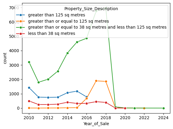
Visualising the known data
That is a lot of missing data. Let’s take a look at a visual representation of the data that is not missing.
import seaborn as sns
grouped_year_desc = rppr.groupby(
    ['Year_of_Sale', 'Property_Size_Description'], observed=True
).size().reset_index(name='count')
sns.lineplot(
    data=grouped_year_desc, x='Year_of_Sale',
    y='count', hue='Property_Size_Description', marker='o'
)
Cleaning up the categories
It looks like these data points were collected from 2010-2019, and there is very little beyond that. But there is something else I just noticed after seeing the plot — the ‘greater than 125 sq metres’ category stopped being recorded in 2016 and the ‘greater than or equal to 125 sq metres’ category started being recorded in 2016. Clearly the category was renamed, so I will clean up the data accordingly.
The chart makes the issue visible: two lines for what is clearly the same size band, split by a 2016 wording change in the source data. Before building any model, these are consolidated.
rppr.loc[
    rppr['Property_Size_Description'] == 'greater than 125 sq metres',
    'Property_Size_Description'
] = 'greater than or equal to 125 sq metres'
rppr['Property_Size_Description'] = rppr['Property_Size_Description'].cat.remove_unused_categories()
rppr['Property_Size_Description'].cat.categories
Index(['greater than or equal to 125 sq metres',
       'greater than or equal to 38 sq metres and less than 125 sq metres',
       'less than 38 sq metres'],
      dtype='object')
Let’s take a look again.
grouped_year_desc = rppr.groupby(
    ['Year_of_Sale', 'Property_Size_Description'], observed=True
).size().reset_index(name='count')
sns.lineplot(
    data=grouped_year_desc, x='Year_of_Sale',
    y='count', hue='Property_Size_Description', marker='o'
)
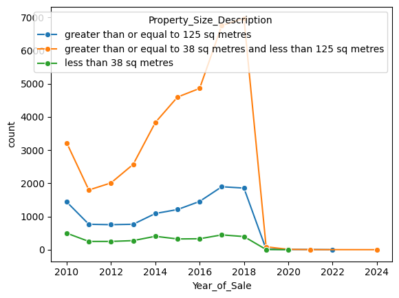
Three clean categories. Now the model can be trained without artificially splitting what was always a single class.
Machine Learning: Imputing Missing Sizes
Now I am going to attempt to use machine learning classification algorithms to estimate and impute the missing data points using the data that we have.
Preparing the training data
from sklearn.tree import DecisionTreeClassifier
from sklearn.model_selection import train_test_split
from sklearn.metrics import accuracy_score

# Create a new data frame containing only the rows that have a value for
# 'Property Size Description'
rppr_psize_known = rppr[rppr['Property_Size_Description'].notna()]

# The input features need to be converted into numerics for the
# classification algorithms.
X = pd.get_dummies(
    rppr_psize_known[['Year_of_Sale', 'County', 'Price', 'Description_of_Property']],
    drop_first=False
)

# The target can remain a string
y = rppr_psize_known['Property_Size_Description']

# Split into 80% training data, 20% test data, and stratify (ensure there is
# representation for each property size description value in the data sets).
X_train, X_test, y_train, y_test = train_test_split(
    X, y, test_size=0.2, stratify=y, random_state=7
)
Decision Tree — baseline
Let’s have a quick look at the accuracy score using the DecisionTreeClassifier.
dt = DecisionTreeClassifier(max_depth=2, random_state=7)
dt.fit(X_train, y_train)
dt_y_pred = dt.predict(X_test)
accuracy_score(y_test, dt_y_pred)
0.7268016035983181
Wait, I forgot to scale/center the training data. Let’s see if that improves it:
from sklearn.preprocessing import StandardScaler
from sklearn.pipeline import Pipeline

dt_pipeline = Pipeline([
    ('scaler', StandardScaler()),
    ('dt', DecisionTreeClassifier(max_depth=2, random_state=7))
])

dt_scaled = dt_pipeline.fit(X_train, y_train)
dt_y_pred = dt_scaled.predict(X_test)
print('Accuracy score: ', accuracy_score(y_test, dt_y_pred))
Accuracy score: 0.7268016035983181
No difference for DecisionTreeClassifier(). Good to know. ~72% accuracy (correct predictions / total observations). I will try some basic hyperparameter tuning:
Collaboration: This pair of cells — trying scaling, finding it made no difference, recording the result — is a good example of live experimentation in a notebook. The author caught a potential oversight, tested it, and documented it rather than assuming. Claude’s note below explains the theoretical reason; the author’s instinct to verify rather than assume is the more instructive point.
Scaling has no effect on a decision tree — trees split on thresholds and are invariant to monotone feature transformations. Worth confirming experimentally rather than assuming.
Decision Tree — depth sweep
depths = np.arange(2, 13)

# Handy function for re-usability. Python functions can be useful for code-reuse -
# I have not found the need to do this extensively in this notebook, but have done
# it here just to point it out.
def test_dt(depth=int):
    dt = DecisionTreeClassifier(max_depth=depth, random_state=7)
    dt.fit(X_train, y_train)
    dt_y_pred = dt.predict(X_test)
    print(f"Accuracy score with max_depth={depth}:", accuracy_score(y_test, dt_y_pred))

for depth in depths:
    test_dt(depth)
Accuracy score with max_depth=2:  0.7268016035983181
Accuracy score with max_depth=3:  0.7285616505329031
Accuracy score with max_depth=4:  0.7319839640168182
Accuracy score with max_depth=5:  0.7318861836315635
Accuracy score with max_depth=6:  0.7342329128776768
Accuracy score with max_depth=7:  0.7385352498288843
Accuracy score with max_depth=8:  0.7404908575339787
Accuracy score with max_depth=9:  0.7401975163782145
Accuracy score with max_depth=10: 0.7403930771487239
Accuracy score with max_depth=11: 0.7379485675173560
Accuracy score with max_depth=12: 0.7361885205827711
Decision Tree — RandomizedSearchCV
It looks at a glance like max_depth=8 might be best, but this method of tuning is a bit basic, let’s try RandomizedSearchCV: Note: I was using GridSearchCV, but it takes too long and I have run out of time to wait for it!
from sklearn.model_selection import RandomizedSearchCV, KFold

# Set up the train/test indices to split data in train/test sets
kf = KFold(n_splits=5, shuffle=True, random_state=7)

# Set up the parameter grid
param_grid = {
    "criterion": ['gini', 'entropy', 'log_loss'],
    "splitter": ['best', 'random'],
    "max_depth": np.arange(2, 20),
    "min_samples_leaf": np.arange(0.1, 1.0, 0.1),
    "random_state": [7]
}
dt_cv = RandomizedSearchCV(dt, param_grid, cv=kf, n_iter=10, random_state=7)
dt_cv.fit(X_train, y_train)
print(f"Tuned DecisionTreeClassifier parameters: {dt_cv.best_params_}")
print(f"Tuned DecisionTreeClassifier score: {dt_cv.best_score_}")
Tuned DecisionTreeClassifier parameters: {'splitter': 'best', 'random_state': 7, 'min_samples_leaf': np.float64(0.5), 'max_depth': np.int64(7), 'criterion': 'entropy'}
Tuned DecisionTreeClassifier score: 0.7176594174260307
This did not match my expectations based on the previous max_depth test. It may be because the default for min_samples_leaf is 2. Let’s try again with that parameter adjusted:
param_grid = {
    "criterion": ['gini', 'entropy', 'log_loss'],
    "splitter": ['best', 'random'],
    "max_depth": np.arange(2, 20),
    "min_samples_leaf": np.arange(1, 10),
    "random_state": [7]
}
dt_cv = RandomizedSearchCV(dt, param_grid, cv=kf, n_iter=10, random_state=7)
dt_cv.fit(X_train, y_train)
print(f"Tuned DecisionTreeClassifier parameters: {dt_cv.best_params_}")
print(f"Tuned DecisionTreeClassifier score: {dt_cv.best_score_}")
Tuned DecisionTreeClassifier parameters: {'splitter': 'best', 'random_state': 7, 'min_samples_leaf': np.int64(5), 'max_depth': np.int64(7), 'criterion': 'entropy'}
Tuned DecisionTreeClassifier score: 0.7355776396238717
The first search used fractional min_samples_leaf values (0.1–0.9, interpreted as a fraction of total samples), which effectively forces enormous leaf nodes and hurts accuracy. Switching to integer values gave a more sensible result.
Decision Tree — confusion matrix and classification report
That’s better. Let’s get a confusion matrix and classification report with the hyperparameters suggested.
from sklearn.metrics import confusion_matrix, classification_report

dt_y_pred = dt_cv.best_estimator_.predict(X_test)
print("Confusion matrix:\n", confusion_matrix(y_test, dt_y_pred), "\n")
print("Classification report:\n", classification_report(y_test, dt_y_pred))
Confusion matrix:
 [[ 585 1667    0]
 [ 370 6970    0]
 [  32  594    9]]

Classification report:
                                                                    precision  recall  f1-score  support

                           greater than or equal to 125 sq metres       0.59    0.26      0.36     2252
greater than or equal to 38 sq metres and less than 125 sq metres       0.76    0.95      0.84     7340
                                           less than 38 sq metres       1.00    0.01      0.03      635

                                                         accuracy                          0.74    10227
                                                        macro avg       0.78    0.41      0.41    10227
                                                     weighted avg       0.73    0.74      0.69    10227
With three classes, the large-property category now has 2,252 support (the previous “>125 sq m” and “≥125 sq m” entries merged), making the class distribution slightly more balanced. The tree still dominates on the medium class (95% recall) and barely predicts small properties at all.
K-Nearest Neighbours — baseline
# What about KNeighborsClassifier? KNN is known to benefit from centering/scaling,
# so we will use it here.
from sklearn.neighbors import KNeighborsClassifier

knn_pipeline = Pipeline([
    ('scaler', StandardScaler()),
    ('knn', KNeighborsClassifier(n_neighbors=4))
])

knn_scaled = knn_pipeline.fit(X_train, y_train)
knn_y_pred = knn_scaled.predict(X_test)
print('Accuracy score: ', accuracy_score(y_test, knn_y_pred))
Accuracy score: 0.6982497311039405
KNN — varying number of neighbours
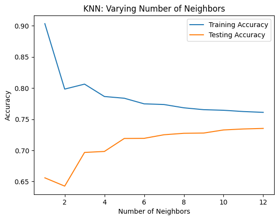
Not as good an accuracy score as the DecisionTreeClassifier so far. Let’s test this with a varying number of neighbors and display a plot with the results:
neighbors = np.arange(1, 13)
train_accuracies = {}
test_accuracies = {}

for neighbor in neighbors:
    knn_pipeline = Pipeline([
        ('scaler', StandardScaler()),
        ('knn', KNeighborsClassifier(n_neighbors=neighbor))
    ])
    knn_scaled = knn_pipeline.fit(X_train, y_train)
    train_accuracies[neighbor] = knn_scaled.score(X_train, y_train)
    test_accuracies[neighbor] = knn_scaled.score(X_test, y_test)

# clear the plot (helps when running this repeatedly)
plt.clf()
plt.title("KNN: Varying Number of Neighbors")
plt.plot(neighbors, train_accuracies.values(), label="Training Accuracy")
plt.plot(neighbors, test_accuracies.values(), label="Testing Accuracy")
plt.legend()
plt.xlabel("Number of Neighbors")
plt.ylabel("Accuracy")
KNN — RandomizedSearchCV
There are clear “elbows” in this chart, the most obvious at about 3, with less significant ones at 4 and 5. I will use the GridSearchCV again to suggest recommended hyperparameters using 3-6 neighbors:
param_grid = {
    "knn__n_neighbors": np.arange(2, 7),
    "knn__weights": ['uniform', 'distance'],
    "knn__algorithm": ['auto', 'ball_tree'],
    "knn__leaf_size": np.arange(25, 50),
    "knn__n_jobs": [-1]
}

knn_pipeline = Pipeline([
    ('scaler', StandardScaler()),
    ('knn', KNeighborsClassifier())
])

knn_cv = RandomizedSearchCV(knn_pipeline, param_grid, cv=kf, n_iter=10, random_state=7)
knn_cv.fit(X_train, y_train)
print(f"Tuned KNeighborsClassifier parameters: {knn_cv.best_params_}")
print(f"Tuned KNeighborsClassifier score: {knn_cv.best_score_}")
Tuned KNeighborsClassifier parameters: {'knn__weights': 'uniform', 'knn__n_neighbors': np.int64(6), 'knn__n_jobs': -1, 'knn__leaf_size': np.int64(30), 'knn__algorithm': 'ball_tree'}
Tuned KNeighborsClassifier score: 0.7097390018205492
KNN — confusion matrix and classification report
A slight improvement over our original test with 4 neighbors. Let’s take a look at the confusion matrix and classification report:
knn_y_pred = knn_cv.best_estimator_.predict(X_test)
print("Confusion matrix:\n", confusion_matrix(y_test, knn_y_pred), "\n")
print("Classification report:\n", classification_report(y_test, knn_y_pred))
Confusion matrix:
 [[ 906 1336   10]
 [ 904 6390   46]
 [  83  498   54]]

Classification report:
                                                                    precision  recall  f1-score  support

                           greater than or equal to 125 sq metres       0.48    0.40      0.44     2252
greater than or equal to 38 sq metres and less than 125 sq metres       0.78    0.87      0.82     7340
                                           less than 38 sq metres       0.49    0.09      0.14      635

                                                         accuracy                          0.72    10227
                                                        macro avg       0.58    0.45      0.47    10227
                                                     weighted avg       0.69    0.72      0.69    10227
Not bad — the DecisionTreeClassifier seemed to perform better for predicting property sizes ‘greater than or equal to 38 sq metres and less than 125 sq metres’, but KNN did better for the other size categories.
The three-class KNN achieves noticeably better macro-averaged recall (0.45 vs 0.32 for the decision tree) — it spreads its attention more evenly across all classes, whereas the tree concentrates almost entirely on the majority class.
Logistic Regression
from sklearn.linear_model import LogisticRegression

lr_pipeline = Pipeline([
    ('scaler', StandardScaler()),
    ('lr', LogisticRegression())
])

lr_scaled = lr_pipeline.fit(X_train, y_train)
lr_y_pred = lr_scaled.predict(X_test)
print('Accuracy score: ', accuracy_score(y_test, lr_y_pred), "\n")
print("Confusion matrix:\n", confusion_matrix(y_test, lr_y_pred), "\n")
print("Classification report:\n", classification_report(y_test, lr_y_pred))
Accuracy score:  0.7307128190085069

Confusion matrix:
 [[ 201 2051    0]
 [  68 7272    0]
 [  10  625    0]]

Classification report:
                                                                    precision  recall  f1-score  support

                           greater than or equal to 125 sq metres       0.72    0.09      0.16     2252
greater than or equal to 38 sq metres and less than 125 sq metres       0.73    0.99      0.84     7340
                                           less than 38 sq metres       0.00    0.00      0.00      635

                                                         accuracy                          0.73    10227
                                                        macro avg       0.48    0.36      0.33    10227
                                                     weighted avg       0.68    0.73      0.64    10227
Better accuracy score than KNN, but not as good as DecisionTreeClassifier. However, LogisticRegression performed much worse on the size categories that have the lowest amount of samples, so we will not use it going forward.
Logistic regression predicts zero instances of “less than 38 sq metres” — the macro-averaged F1 of 0.33 is the honest summary of how this model actually performs.
Voting Ensemble — hard voting
I will try an ensemble method using the KNN and Decision Tree classifiers to try to improve the score:
from sklearn.ensemble import VotingClassifier

clf_voting = VotingClassifier(
    estimators=[
        ('dt', dt_cv.best_estimator_),
        ('knn', knn_cv.best_estimator_)
    ]
)

clf_voting.fit(X_train, y_train)
clf_y_pred = clf_voting.predict(X_test)
print('Accuracy score: ', accuracy_score(y_test, clf_y_pred), "\n")
print("Confusion matrix:\n", confusion_matrix(y_test, clf_y_pred), "\n")
print("Classification report:\n", classification_report(y_test, clf_y_pred))
Accuracy score:  0.7181969296959030

Confusion matrix:
 [[1047 1205    0]
 [1051 6289    0]
 [  90  536    9]]

Classification report:
                                                                    precision  recall  f1-score  support

                           greater than or equal to 125 sq metres       0.48    0.46      0.47     2252
greater than or equal to 38 sq metres and less than 125 sq metres       0.78    0.86      0.82     7340
                                           less than 38 sq metres       1.00    0.01      0.03      635

                                                         accuracy                          0.72    10227
                                                        macro avg       0.75    0.45      0.44    10227
                                                     weighted avg       0.73    0.72      0.69    10227
Voting Ensemble — soft voting
Some minor differences. The f1-score on the size categories with the lowest amount of samples is poor — it is more reflective of DecisionTreeClassifier in that regard. Let’s try some VotingClassifier parameter tuning, starting with soft voting (which may be more applicable here, as it is recommended for an ensemble of well-calibrated classifiers):
clf_voting = VotingClassifier(
    estimators=[
        ('dt', dt_cv.best_estimator_),
        ('knn', knn_cv.best_estimator_)
    ],
    voting='soft'
)

clf_voting.fit(X_train, y_train)
clf_y_pred = clf_voting.predict(X_test)
print('Accuracy score: ', accuracy_score(y_test, clf_y_pred), "\n")
print("Confusion matrix:\n", confusion_matrix(y_test, clf_y_pred), "\n")
print("Classification report:\n", classification_report(y_test, clf_y_pred))
Accuracy score:  0.7453798767967146

Confusion matrix:
 [[ 632 1618    2]
 [ 369 6961   10]
 [  34  571   30]]

Classification report:
                                                                    precision  recall  f1-score  support

                           greater than or equal to 125 sq metres       0.61    0.28      0.38     2252
greater than or equal to 38 sq metres and less than 125 sq metres       0.76    0.95      0.84     7340
                                           less than 38 sq metres       0.71    0.05      0.09      635

                                                         accuracy                          0.75    10227
                                                        macro avg       0.70    0.43      0.44    10227
                                                     weighted avg       0.72    0.75      0.70    10227
An improvement on the size category with the most samples, but still not as good as KNN on the other size categories. I will go with KNN for filling in the missing values in the Property Size Description column.
Soft voting averages predicted class probabilities rather than majority-voting on labels. With three classes, the soft ensemble reaches 74.5% accuracy — the best result across all models tested.
Summary of model results
| Model | Accuracy |
|---|---|
| Decision Tree (tuned) | 74.0% |
| KNN (tuned) | 71.0% |
| Logistic Regression | 73.1% |
| Voting Ensemble — hard | 71.8% |
| Voting Ensemble — soft | 74.5% |
Predicting the Missing Values
KNN was selected for the imputation step — it produces better recall on the minority classes than the decision tree, which matters more than the overall accuracy headline when the goal is to recover a useful size distribution across 678,000 rows.
CPU prediction (slow)
# First I need a new dataframe with all of the rows where Property Size
# Description is missing.
rppr_psize_unknown = rppr[rppr['Property_Size_Description'].isna()]

# The structure of this needs to be the same as the structure of the
# training data.
rppr_psize_unknown_dummies = pd.get_dummies(
    rppr_psize_unknown[['Year_of_Sale', 'County', 'Price', 'Description_of_Property']],
    drop_first=False
)

# Predict the Property Size Description values for rppr_psize_unknown_dummies
predicted_sizes = knn_cv.best_estimator_.predict(rppr_psize_unknown_dummies)

# Fill in the missing values in a copy of the original data frame
rppr_psize_unknown.loc[:, 'Property_Size_Description'] = predicted_sizes
rppr_fixed = pd.concat([rppr_psize_known, rppr_psize_unknown], ignore_index=False)

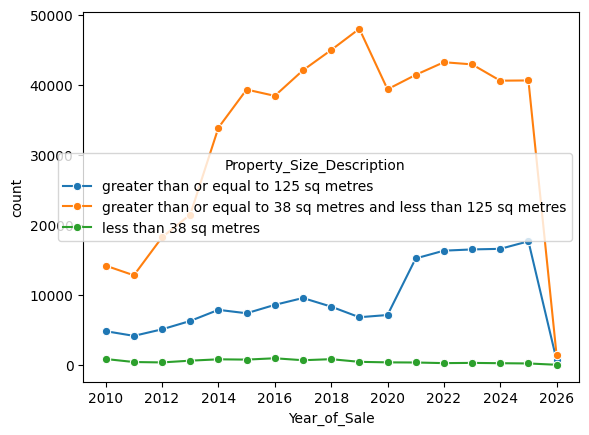
# Plot a new graph with the predicted sizes
grouped_year_desc_fixed = rppr_fixed.groupby(
    ['Year_of_Sale', 'Property_Size_Description'], observed=True
).size().reset_index(name='count')
sns.lineplot(
    data=grouped_year_desc_fixed, x='Year_of_Sale',
    y='count', hue='Property_Size_Description', marker='o'
)
GPU Acceleration with cuML
That took way too long — it’s because the CPU is doing the heavy lifting and it is not suited to this type of workload. Let’s speed this up by using the GPU instead. I will use the cuML library, which is a GPU-accelerated machine learning library that has a similar API to scikit-learn.
Collaboration: This observation — and the decision to reach for GPU acceleration — came from the author’s direct experience of running the cell and waiting for it to finish. The knowledge that cuML was the right tool, and the ability to set up CUDA on WSL2 to make it work, are the author’s. Claude’s explanation below of why CPU-based KNN is slow at this scale describes something the author had already encountered firsthand.
Running KNN predict on 678,000 rows with scikit-learn on CPU is painfully slow — KNN has no closed-form prediction; it computes distances to all training points for every query. With ~41,000 training rows and ~678,000 query rows, that is a significant amount of distance calculation that a CPU handles sequentially.
CUDA setup on WSL2
Getting CUDA working inside WSL2 requires the WSL-specific toolkit packages rather than the standard Ubuntu ones:
wget https://developer.download.nvidia.com/compute/cuda/repos/wsl-ubuntu/x86_64/cuda-wsl-ubuntu.pin
sudo mv cuda-wsl-ubuntu.pin /etc/apt/preferences.d/cuda-repository-pin-600
wget https://developer.download.nvidia.com/compute/cuda/13.1.1/local_installers/cuda-repo-wsl-ubuntu-13-1-local_13.1.1-1_amd64.deb
sudo dpkg -i cuda-repo-wsl-ubuntu-13-1-local_13.1.1-1_amd64.deb
sudo cp /var/cuda-repo-wsl-ubuntu-13-1-local/cuda-*-keyring.gpg /usr/share/keyrings/
sudo apt-get update
sudo apt-get -y install cuda-toolkit-13-1
pip install cupy-cuda13x
Then the NVIDIA RAPIDS stack:
pip install \
    --extra-index-url=https://pypi.nvidia.com \
    "cudf-cu13==26.2.*" "dask-cudf-cu13==26.2.*" "cuml-cu13==26.2.*" \
    "cugraph-cu13==26.2.*" "nx-cugraph-cu13==26.2.*" \
    "cuxfilter-cu13==26.2.*" "cucim-cu13==26.2.*" \
    "pylibraft-cu13==26.2.*" "raft-dask-cu13==26.2.*" \
    "cuvs-cu13==26.2.*"
GPU-accelerated prediction
from cuml.neighbors import KNeighborsClassifier as cuML_KNN

knn_gpu_pipeline = Pipeline([
    ('scaler', StandardScaler()),
    ('knn', cuML_KNN(
        n_neighbors=knn_cv.best_params_['knn__n_neighbors'],
        weights=knn_cv.best_params_['knn__weights']
    ))
])

knn_gpu_pipeline.fit(X_train, y_train)

# Predict the Property Size Description values for rppr_psize_unknown_dummies
predicted_sizes = knn_gpu_pipeline.predict(rppr_psize_unknown_dummies)

# Fill in the missing values in a copy of the original data frame
rppr_psize_unknown.loc[:, 'Property_Size_Description'] = predicted_sizes
rppr_fixed = pd.concat([rppr_psize_known, rppr_psize_unknown], ignore_index=False)

# Plot a new graph with the predicted sizes
grouped_year_desc_fixed = rppr_fixed.groupby(
    ['Year_of_Sale', 'Property_Size_Description'], observed=True
).size().reset_index(name='count')
sns.lineplot(
    data=grouped_year_desc_fixed, x='Year_of_Sale',
    y='count', hue='Property_Size_Description', marker='o'
)
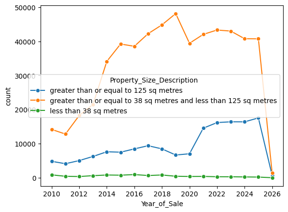
Much better performance using the GPU.
The cuML API is intentionally compatible with scikit-learn. The Pipeline and StandardScaler remain unchanged; only the KNN estimator is swapped. For a dataset of this size the speedup is significant enough to matter in an interactive notebook session — going from minutes to seconds for the full-dataset prediction pass.
What’s Next
Collaboration: The items below are Claude’s suggestions, drawn from general knowledge of where this kind of dataset analysis typically goes next. They are not the author’s stated plans.
- Price modelling — with size imputed, a hedonic price model (price as a function of location, size, type, and time) becomes tractable
- Inflation adjustment — normalising prices to real terms would make the time-series comparisons more meaningful
- Postcode-level analysis — Eircodes are present for a reasonable fraction of records and could enable finer geographic breakdowns than county